Credit Risk Analysis of a Corporate Bond Portfolio


Background
This is a brief overview of my senior capstone project for Souther New Hampshire University's MAT430 Seminar in Applied Mathematics. The purpose of this article is to showcase the underlying code and less of the core mathematics. More information on the topic can be found on my full report at the link above.
Credit rating agencies publish historical corporate rating transition matrics on an annual basis. This project compares a continous time Markov approximation versus the standard discrete time Markov chain when forecasting credit risk. The project is split into two parts: a comparison of cumulative default rates across each credit rating and a portfolio level analysis comparing credit Value at Risk (VaR).
Initialization
The transition matrix published by S&P Global included a Not Rated (NR) column. To resolve this, the NR column is filtered using
Loading the S&P Global matrix and running the filtering gives us the base discrete matrix with default as the absorbing state.
P = 8×8
                  0.900537                  0.092035                  0.005262                   0.00031                  0.001032                   0.00031                  0.000515                         0
                  0.004675                   0.91149                  0.077914                  0.004571                  0.000519                  0.000613                  0.000208                  0.000218
                  0.000208                  0.015423                  0.931847                  0.048353                  0.002297                  0.001042                  0.000104                  0.000621
                         0                  0.000742                  0.032347                  0.926185                  0.034044                  0.004242                  0.000955                  0.001485
                   0.00011                   0.00022                  0.001102                  0.048915                   0.86912                  0.068855                  0.005508                  0.006169
                         0                  0.000228                  0.000685                  0.001598                  0.051033                  0.858317                  0.054687                  0.033451
                         0                         0                  0.000824                   0.00153                  0.004708                  0.155114                  0.530423                  0.307403
                         0                         0                         0                         0                         0                         0                         0                         1
Generator Matrix
In a continuous Markov model, transitions are modeled based on the Kolmogorov forward equation solved via . However, because the S&P base matrix contains zero probability entries for transitions accessible through multi-step jumps (ex. AAA D in a single year), no generator matrix exists for .
Therefore, we must approximate the matrix . This project use Jarrow et al.'s logarithmic approach.
n = size(P, 1);
Q = zeros(n, n);

for i = 1:n
    p_ii = log(P(i,i));
    Q(i, i) = p_ii;
    for j = 1:n
        if i ~= j
            Q(i, j) = P(i, j) * p_ii / (P(i, i) - 1);
        end
    end
end
Q(8,:) = 0;
round(Q,4)
ans = 8×8
   -0.1048    0.0969    0.0055    0.0003    0.0011    0.0003    0.0005         0
    0.0049   -0.0927    0.0816    0.0048    0.0005    0.0006    0.0002    0.0002
    0.0002    0.0160   -0.0706    0.0501    0.0024    0.0011    0.0001    0.0006
         0    0.0008    0.0336   -0.0767    0.0354    0.0044    0.0010    0.0015
    0.0001    0.0002    0.0012    0.0524   -0.1403    0.0738    0.0059    0.0066
         0    0.0002    0.0007    0.0017    0.0550   -0.1528    0.0590    0.0361
         0         0    0.0011    0.0021    0.0064    0.2095   -0.6341    0.4151
         0         0         0         0         0         0         0         0
We then calculate the continuous using
P_t = expm(Q)
P_t = 8×8
    0.9008    0.0879    0.0087    0.0007    0.0010    0.0004    0.0004    0.0001
    0.0044    0.9123    0.0753    0.0063    0.0007    0.0007    0.0002    0.0003
    0.0002    0.0148    0.9332    0.0467    0.0030    0.0012    0.0001    0.0007
    0.0000    0.0010    0.0313    0.9278    0.0319    0.0052    0.0009    0.0019
    0.0001    0.0003    0.0019    0.0472    0.8717    0.0645    0.0057    0.0086
    0.0000    0.0002    0.0008    0.0029    0.0478    0.8646    0.0404    0.0432
    0.0000    0.0000    0.0009    0.0018    0.0087    0.1433    0.5343    0.3110
         0         0         0         0         0         0         0    1.0000
Cumulative Default Rates
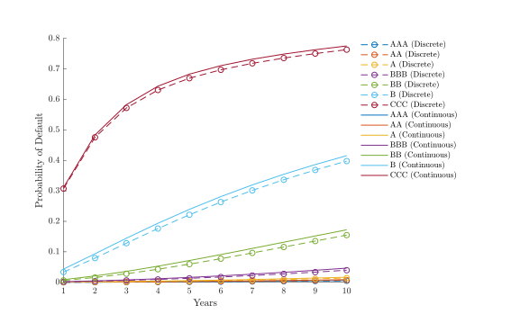
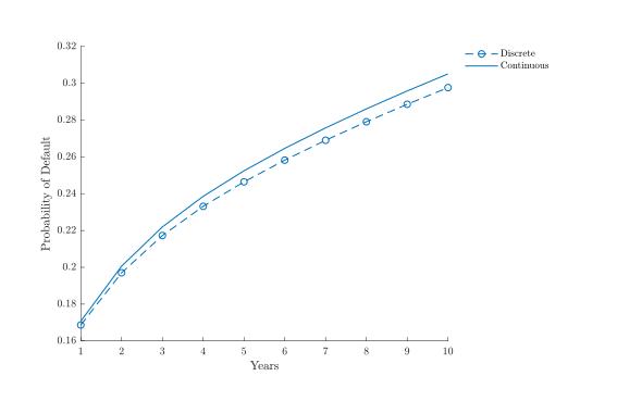
Under the discrete model, future rating transitions are modeled as . In the continuous model, they are calculated using the forward equation from above. We can calculate the cumulative default rate by tracking states as they approach the absorbing default state.
states = size(P, 1);
cumPD_disc = zeros(states, steps);
cumPD_cont = zeros(states, steps);

meanPD_disc = zeros(1, steps);
meanPD_cont = zeros(1, steps);

for t = 1:steps
    P_disc = P^t;
    P_cont = expm(Q * t);

    cumPD_disc(:, t) = P_disc(:, end);
    cumPD_cont(:, t) = P_cont(:, end);

    % Column-wise mean probability of default
    meanPD_disc(t) = mean(cumPD_disc(:, t));
    meanPD_cont(t) = mean(cumPD_cont(:, t));
end
mean_diff = meanPD_cont - meanPD_disc
mean_diff = 1×10
       0.00206385086275396       0.00359673781864858        0.0046831177555938       0.00544865950879336       0.00600009594508505       0.00641400372899986       0.00674105728670771       0.00701331150783535       0.00725053495067174       0.00746478031953929
CreditMetrics Monte Carlo Simulation
To quantify portfolio level loss, we apply the CreditMetrics framework developed by the RiskMetrics group. This method correlates rating migrations through a company's stock asset returns.
Asset Returns
Using the Yahoo Finance yfinance Python package, we can download annual stock data for each company in the portfolio.
try:
    data = yf.download(tickers, start=start_date, end=end_date, progress=True)

    print(f"Downloaded data columns: {data.columns.tolist()}")
    print(f"Downloaded data shape: {data.shape}")

    if isinstance(data.columns, pd.MultiIndex):
        if 'Adj Close' in data.columns.get_level_values(0):
            adj_close = data['Adj Close']
        else:
            adj_close = data['Close']
    else:
        if 'Adj Close' in data.columns:
            adj_close = data[['Adj Close']].copy()
            adj_close.columns = tickers
        else:
            adj_close = data[['Close']].copy()
            adj_close.columns = tickers

except Exception as e:
    print(f"Error downloading data: {e}")
From this data we then calculate the annual return percentage as and write this to a Pandas dataframe.
def calculate_annual_returns(prices_df):
    """
    Calculate annual returns for each stock
    Returns a DataFrame with years as index and tickers as columns
    """
    annual_returns = pd.DataFrame()

    years = sorted(prices_df.index.year.unique())

    for year in years:
        if year < 2015 or year > 2025:
            continue

        year_data = prices_df[prices_df.index.year == year]

        if len(year_data) < 2:
            continue

        # Get first and last price of the year
        first_price = year_data.iloc[0]
        last_price = year_data.iloc[-1]

        # Calculate annual return: (end_price - start_price) / start_price * 100
        year_returns = ((last_price - first_price) / first_price * 100).round(2)

        annual_returns[year] = year_returns

    return annual_returns.T

returns_df = calculate_annual_returns(adj_close)
Saving that as a CSV we can then access our annual stock returns in MATLAB.
stock_returns = readmatrix("annual_stock_returns_2015_2025.csv");
stock_returns = stock_returns(:, 2:end)
stock_returns = 11×33
-23.38 -16.44 29.51 2.07 -4.35 2.07 -4.83 0.51 -24.19 -18.64 0.37 -16.12 -14.07 -16.44 -14.07 -11.13 18.64 43.3 -16.55 -6.07 -14.48 1.72 7.29 -8.57 -24.19 0.69 7.83 -28.86 2.07 46.77 6.47 -63.2 -18.64
45.82 8.77 18.75 7.51 17.31 7.51 36.62 32.51 11.73 34.79 18.8 36.24 33.02 8.77 33.02 39.29 39.81 47.65 37.5 37.28 17.75 9.71 28.72 11.66 11.73 -0.19 38.7 9.69 7.51 26.14 5.5 39.46 34.79
18.98 24.13 22.16 11.41 24.59 11.41 33.1 8.75 33.92 23.14 35.23 14.82 21.82 24.13 21.82 53.33 38.61 8.9 24.25 6.79 17.83 21.43 24.88 17.97 33.92 10.82 25.39 10.91 11.41 46.88 14.08 -14.29 23.14
-19.92 -1.62 12.76 -22.37 -28.44 -22.37 -16.08 -10.6 -2.26 -13.6 15.11 -16.18 -12.58 -1.62 -12.58 -3.82 14.16 -0.67 -22.35 -33.76 -15.05 -16.7 -17.17 40.7 -2.26 -6.69 -7.5 14.73 -22.37 -0.3 24.07 -14.63 -13.6
16.51 19.16 60.13 19.22 53.49 19.22 44.32 31.31 32.02 18.3 46.04 19.9 16.19 19.16 16.19 19.15 22.78 20.17 30.21 36.41 41.4 13.37 38.65 22.9 32.02 22.48 44.75 4.9 19.22 29.44 -6.05 40.59 18.3
1.28 22.02 -1.44 -41.59 -21.03 -41.59 -12.67 -11.71 -2.55 7.74 31.99 3.15 4.81 22.02 4.81 54.74 21.86 71.59 35.65 15.25 -23.68 12.76 -3.22 12.13 -2.55 12.27 -6.67 -36.46 -41.59 42.02 3.17 -30.34 7.74
41.63 38.91 -7.26 63.75 3.48 63.75 51 28.09 40.21 34.42 28.26 48.8 41.65 38.91 41.65 29.54 45.69 -12.42 47.08 46.89 28.81 44.73 38.05 58.37 40.21 24.23 28.96 88.58 63.75 61.13 66.7 24.76 34.42
-28.58 -5.39 -6.09 -16.7 -25.44 -16.7 -26.61 -25.87 -11.02 -8.8 -6.85 -13.34 -13.42 -5.39 -13.42 23.98 6.91 22.35 -12.16 -10.85 18.76 -44.76 -21.6 -4.59 -11.02 -24.83 -14.45 67.99 -16.7 -13 -6.61 17.6 -8.8
7.24 27.84 31.25 21.47 17.55 21.47 3.61 -9.85 29.22 12.62 -25.5 14.07 5.55 27.84 5.55 -4.48 3.04 15.82 13 14.95 -14.34 7.35 1.7 12.31 29.22 36.53 29.64 6.38 21.47 106.27 -41.29 4.52 12.62
18.54 62.1 54.36 46.15 37.65 46.15 32.95 21.77 59.49 23.3 19.83 4.08 -12.93 62.1 -12.93 7.28 -4.74 38.34 38.76 51.04 38.98 49.3 28.03 9.87 59.49 10.09 42.63 -13.3 46.15 116.48 -5.31 62.68 23.3
Forward Rates & Pricing
If a bond migrates to a different credit rating, its market value changes to reflect the yield curve of that new rating. Implied forward rates are calculates using spot rates for each credit rating across maturities. A comprehensive overview of this can be found in Hull's Risk Management and Financial Institutions.
function forward_rates = forward_curves(prices, FV, ratings)
    % Inputs:
    % - prices: m x n matrix (m = # ratings, n = maturities)
    % - FV: face value
    % - ratings: cell array of rating names (m x 1)

    [m, n] = size(prices); % n maturities (e.g., 5 for 1- to 5-year bonds)

    % Compute spot rates for each rating and year
    spot_rates = (FV ./ prices).^(1 ./ (1:n)) - 1;  % m x n

    % Preallocate forward rate table: F12, F13, ..., F1n
    forward_rates = zeros(m, n-1);  % We'll compute F1j for j = 2 to n

    % Compute forward rates starting from year 1 to year j
    for j = 2:n
        s1 = spot_rates(:,1);   % spot rate for year 1
        sj = spot_rates(:,j);   % spot rate for year j

        f1j = ((1 + sj).^j ./ (1 + s1)).^(1 / (j - 1)) - 1;
        forward_rates(:, j-1) = f1j;  % Convert to percentage
    end

    varNames = arrayfun(@(j) sprintf('F1%d', j), 2:n, 'UniformOutput', false);
    forward_table = array2table(forward_rates, 'VariableNames', varNames);
    forward_table = addvars(forward_table, ratings(:), 'Before', 1, 'NewVariableNames', 'Rating')
end
forward_table =
    Rating       F12         F13         F14         F15
    _______    ________    ________    ________    ________

    {'AAA'}    0.043478    0.044466      0.0414    0.040194
    {'AA' }    0.055866    0.054403    0.054902    0.055977
    {'A'  }    0.062147    0.064204     0.06417    0.063433
    {'BBB'}    0.068966    0.071517     0.07196    0.073609
    {'BB' }    0.076471    0.079632    0.083169    0.083053
    {'B'  }    0.084337    0.088214    0.092608    0.093265
    {'CCC'}         0.1     0.10554     0.10911     0.10512
Using these forward rates, each bond's future cash flow is revalued across all possible credit ratings. In the event of a default, bonds are assigned an arbitrary 51% recovery rate.
function values = forward_value(bonds, num_years, forward_rates)
    num_bonds = length(portfolio);
    values = zeros(8, num_bonds);
    for i = 1:num_bonds
        for j = 1:7
            F_A = forward_rates(j, :);
            values(j, i) = bond_value(bonds(i).coupon * 100, F_A, num_years);
        end
        values(8, i) = 51.00;
    end
end

function Vx_A = bond_value(Cx, F_A, n)
    current = 0;
    for i = 1:n
        numerator = Cx;
        denominator = (1 + F_A(i))^(i - 1);
        current = current + (numerator / denominator);
    end

    numerator = Cx + 100;
    denominator = (1 + F_A(n))^n;
    Vx_A = current + (numerator / denominator);
end
forward_values = 8×33
  105.1354   99.0646  102.1000  104.7242  102.1000  101.7083   98.1775   98.3145  106.8881  102.9323  104.8906  105.0375  105.0238  102.1979  105.9305  105.1354  106.1146  105.5271  104.0779  104.6106  103.9115  107.1917  106.7647  103.9115  106.1773  104.7437  107.7537  105.0375  106.0127  104.3521  104.9396  105.9188  104.9396
  103.9577   97.9217  100.9397  103.5488  100.9397  100.5503   97.0397   97.1760  105.7003  101.7672  103.7143  103.8603  103.8467  101.0370  104.7482  103.9577  104.9312  104.3471  102.9062  103.4359  102.7407  106.0021  105.5777  102.7407  104.9935  103.5683  106.5609  103.8603  104.8300  103.1788  103.7630  104.7365  103.7630
  103.3710   97.3524  100.3617  102.9633  100.3617   99.9734   96.4729   96.6088  105.1086  101.1868  103.1283  103.2739  103.2603  100.4588  104.1593  103.3710  104.3418  103.7593  102.3226  102.8507  102.1576  105.4096  104.9863  102.1576  104.4039  102.9827  105.9668  103.2739  104.2408  102.5944  103.1769  104.1476  103.1769
  102.7419   96.7419   99.7419  102.3355   99.7419   99.3548   95.8652   96.0006  104.4742  100.5645  102.5000  102.6452  102.6316   99.8387  103.5277  102.7419  103.7097  103.1290  101.6968  102.2232  101.5323  104.7742  104.3523  101.5323  103.7716  102.3548  105.3297  102.6452  103.6090  101.9677  102.5484  103.5161  102.5484
  102.0587   96.0790   99.0689  101.6537   99.0689   98.6831   95.2051   95.3402  103.7852   99.8887  101.8176  101.9623  101.9488   99.1653  102.8419  102.0587  103.0232  102.4445  101.0171  101.5418  100.8531  104.0842  103.6636  100.8531  103.0850  101.6730  104.6378  101.9623  102.9229  101.2872  101.8658  102.8303  101.8658
  101.3528   95.3939   98.3733  100.9491   98.3733   97.9889   94.5231   94.6577  103.0732   99.1903  101.1125  101.2567  101.2432   98.4694  102.1332  101.3528  102.3139  101.7372  100.3148  100.8376  100.1514  103.3711  102.9521  100.1514  102.3754  100.9683  103.9228  101.2567  102.2139  100.5839  101.1606  102.1217  101.1606
   99.9773   94.0591   97.0182   99.5764   97.0182   96.6364   93.1943   93.3279  101.6859   97.8295   99.7386   99.8818   99.8685   97.1136  100.7524   99.9773  100.9318  100.3591   98.9464   99.4656   98.7841  101.9818  101.5656   98.7841  100.9929   99.5955  102.5297   99.8818  100.8325   99.2136   99.7864  100.7409   99.7864
   51.0000   51.0000   51.0000   51.0000   51.0000   51.0000   51.0000   51.0000   51.0000   51.0000   51.0000   51.0000   51.0000   51.0000   51.0000   51.0000   51.0000   51.0000   51.0000   51.0000   51.0000   51.0000   51.0000   51.0000   51.0000   51.0000   51.0000   51.0000   51.0000   51.0000   51.0000   51.0000   51.0000
Z-Threshold Matrix
To determine which rating a bond migrates to, we map the cumulative transition probabilities of into standard normal thresholds with the inverse normal CDF.
function Z = threshold_matrix(P)

    Z = zeros(8, 7);

    for i = 1:7
        cumprobs = cumsum(P(i, :));
        z_scores = -norminv(cumprobs);
        z_thresholds = [Inf, z_scores(1:7)];
        Z(:, i) = z_thresholds';
    end
end
Z_matrix = 8×7
       Inf       Inf       Inf       Inf       Inf       Inf       Inf
   -1.2846    2.5990    3.5297       Inf    3.6949       Inf       Inf
   -2.4359   -1.3797    2.1537    3.1778    3.4057    3.5054       Inf
   -2.8529   -2.5168   -1.6209    1.8372    2.9820    3.1172    3.1473
   -2.9017   -3.0000   -2.6381   -1.7423    1.6415    2.8056    2.8264
   -3.1473   -3.1448   -2.8990   -2.4739   -1.4015    1.6114    2.4541
   -3.2827   -3.5173   -3.1452   -2.8149   -2.2676   -1.3523    0.9856
       NaN   -4.2649   -3.1841   -2.9708   -2.5023   -1.8323   -0.5032
Monte Carlo Simulation
We draw 10,000 joint return samples from the multivariate normal distribution given by the stock return mean and covariance.
function samples = simulate_returns(n, stock_returns)
    % Generate n vectors (length of # of bonds) by sampling from
    % multivariate normal distribution using mean and covariance
    mean_vector = mean(stock_returns);
    covariance_matrix = cov(stock_returns);
    distribution = mvnrnd(mean_vector, covariance_matrix, n);

    % Standardize using Z score
    samples = zscore(distribution);
end
samples = 10000×33
          1.78269512560902         0.723546783145017          0.25837331537889         -0.73376240984272          1.05316412051832        -0.733762409842721         0.841985756017794          1.15431050466882         0.342240945953681          1.66082972335126          1.06660274744582          1.31883612159334           1.4850350329852         0.723546783145016           1.4850350329852          1.80726598327502         0.288245342286239           1.8785552711381          1.81878391241117          1.20541554782135        -0.368001915089055          0.95050416744231         0.928784656607177        -0.259160965409003          0.34224094595368         0.731586242479586          1.18160584272539          -2.0395955095996        -0.733762409842719         0.391591205855048         -0.88382227110433         0.246604617360242          1.66082972335126
        -0.173233400063149        -0.834084886701058         0.979012140824063        -0.565150921926263        -0.775926297509358        -0.565150921926263        -0.270860510249718        -0.823636643984834       -0.0797782746733463        -0.195415119869276        -0.142084720414592        -0.370073894061075         -1.28486909141412        -0.834084886701058         -1.28486909141412          0.25512554427305          2.01354041984799          1.20847495334925         0.147446493574243        -0.285268083855757         -1.42699861193326         0.111316941285265        0.0161264086553301         -1.11944094130011       -0.0797782746733455           1.6467982783219        -0.504882397126105        0.0702063435157641        -0.565150921926262          1.04065832362093        -0.397513628922442        -0.808116746048499        -0.195415119869273
         -1.13785086882664         -1.17014248639927         0.142676096324045         0.415186719746835        -0.972398371801302         0.415186719746835        -0.590078025435152         -0.46132720777622         -0.79472604948997         -1.54582921197369         -1.03868295137535        -0.799454838956419        -0.931240058411148         -1.17014248639927        -0.931240058411148         -2.42314254458177          0.13884124692298         -1.33560976022493         -1.70110244601852         -1.20268586207159        -0.991714236702651        -0.462734109685344         -0.58086441551619         0.833620517163103         -0.79472604948997         0.316729753765828        -0.638948755895182         0.680240744733055         0.415186719746834       -0.0528231516138454         0.843505911577651         -1.03758240379879         -1.54582921197369
        -0.600923404403156          0.16868541740609          1.29251876689519          0.80048873573297          1.08115403693742          0.80048873573297          0.35863319449587       -0.0440071453289877         0.570910775260922        -0.555023347777636       -0.0760507128990874        -0.352937344942301        -0.392271607351268          0.16868541740609        -0.392271607351268         -1.19185308880125        -0.262564444362731         -0.92375092911883        -0.428873991272158        -0.130781409079203     -0.000507706396740498         0.478702872471656         0.518242663316849        0.0526868379170118         0.570910775260922          1.55366482991857         0.614538139143261        -0.368793473083446         0.800488735732969         0.996946510066453        -0.576340951683975        -0.715782243319377        -0.555023347777634
          1.67524517470301          1.09075708723357         0.548812148263738            1.002926774173          1.16761142162095            1.002926774173          1.51552002740992           1.6098849789129          1.31852723763692          1.84445512075846          1.04633936555792          1.53250622935482         0.832255139460636          1.09075708723357         0.832255139460636          1.03991639391891         0.504635061503457          0.52216511585863          1.87963500688405          2.06425892082203          1.96501427106835          0.81431338962732          1.47816949325495         0.131406550689142          1.31852723763693         0.206374336259998          1.37903919775771          0.88260442542318          1.00292677417301         0.207669950196683         0.125969103824492           2.4250309617051          1.84445512075846
        -0.920486474057084         -1.22054030110202         0.232118690669919        -0.957962470125433        -0.833132171650605        -0.957962470125434         -1.37218455203711         -1.50908311512644         -1.01231441778864        -0.942254690049662         -2.14866959633249         -1.03083646438064         -1.21754734258488         -1.22054030110202         -1.21754734258488        -0.787095863947957       -0.0135468650691655         0.947988278699785         -1.18002160789343         -1.10722519294382         -1.67460722799491         -1.20545555617665         -1.29372546397734         -1.89055446428883         -1.01231441778864        0.0276921263017059        -0.684394528481579        -0.518140278814966        -0.957962470125432         0.460428262772991         -1.77157082894655        -0.899442124347108        -0.942254690049661
         0.997761798278749        -0.407357001804833         0.274899730834174         0.465123472085194        0.0833832598000949         0.465123472085194         0.616051232784355          1.01760660201645        -0.490079862672661         0.582478406826223        -0.349113691765166          0.95339578535417         0.441786339023194        -0.407357001804833         0.441786339023194        -0.195802573314857         0.945453011113332          1.59527899218269         0.867153608005862          1.19440676403666        -0.581922368978074         0.849532008573636         0.995552803320755        -0.766217498536484         -0.49007986267266         0.848903263713611         0.735391402967954        -0.609581949839986         0.465123472085194         0.887202120926126         0.103237648332947         -0.28613356692312         0.582478406826223
          1.50715894482493          1.26857551153605         0.252719593527241          1.16233107320881          1.12576329210321          1.16233107320881          1.84970891386456          2.62618745209575         0.851030510721784          1.14201745846148          2.38410315105574          0.93875470249905          1.15963823174255          1.26857551153605          1.15963823174254          0.38394903473276       -0.0323724432378589        0.0466565232362614          1.30074243371034          1.46151306409397          1.54342388915997          2.11730276795412          1.91427764158095          1.47779580102719         0.851030510721784        -0.672411853952295          1.35545769335664        -0.955288140879117          1.16233107320881      -0.00906856451547339          2.17641841963567         0.712521812084847          1.14201745846148
         -1.55527436728891          -1.2655445139132         0.326500982551245       -0.0765868838177484         0.135220024837763       -0.0765868838177483        -0.727968994817738        -0.749021070355577        -0.767479380192113         -1.64169215297833        -0.981809463148842        -0.832012279040352        -0.315714015587592          -1.2655445139132        -0.315714015587592         -2.08524177085212        -0.919793725227976         -2.08796623962502         -2.06581732455832         -1.56216317429884        -0.226957647530187         -1.61272757489352        -0.882074275459313         0.682943288703968        -0.767479380192113        0.0955259029035261        -0.337435626968246         0.598594078774927       -0.0765868838177493         -1.06849041820418          -0.6154267932092        -0.649283067241718         -1.64169215297833
         -0.90520570794572        -0.795081949488289        -0.238969940949545        -0.674818156964313        -0.671568053014494        -0.674818156964313        -0.887498947591842        -0.992407765963265         -0.47170735684897        -0.699326567373067        -0.657663572945116        -0.835190438380303        -0.785380797482688         -0.79508194948829        -0.785380797482687        -0.145611919947746        -0.197467785315996        -0.433475603025332         -1.05189526352602         -1.01235104762858         0.175185413127107         -1.51678335627251         -1.08497329249122        -0.499699434836458         -0.47170735684897         -1.14705489548694        -0.849195222148317         0.961844757771916        -0.674818156964312         -1.04585442527905        -0.474730783158138          0.41886957570541        -0.699326567373068
For each simulated path, each bond's return is compared against the -threshold matrix to determine its migrated rating and looked up in the forward valuation matrix to calculate the total portfolio value.
function result = revaluate_portfolio(portfolio, samples, n, Z, forward_rates)
    initial_ratings = [portfolio.rating];
    num_bonds = length(initial_ratings);
    result = zeros(n, 1);


    for sim = 1:n
        % For each simulation, calculate the new rating
         new_ratings = zeros(1, num_bonds);

        new_values_sum = 0;
        for bond = 1:num_bonds
            raw_return = samples(sim, bond);
            initial_rating = initial_ratings(bond);
            Z_x = Z(:, initial_rating);
            new_rating = 8;

            for rating = 8:-1:1
                thres = Z_x(rating);


                if(isnan(thres))
                    new_rating = rating - 1;
                    continue
                end

                if(raw_return > thres)
                    new_rating = rating - 1;
                end
            end
            new_ratings(bond) = new_rating;

            % Revaluate based on forward curve and new rating
            new_values_sum = new_values_sum + forward_rates(new_rating, bond);
        end
        result(sim) = new_values_sum;
    end
end
simulated_portfolio = 1×10000
            3376.109512256          3370.97794883378           3374.1823502209          3318.98540693711          3325.41813097225          3322.35998166204          3324.20349266802          3325.41813097225          3324.20349266802          3324.82881439074          3323.00887250464          3326.08404002561          3373.56258357711          3370.95948056677          3372.88950055226          3324.20349266802          3324.78987395813          3374.94071489024          3322.26490409899          3373.56258357711          3372.22548895483          3369.77966532105          3323.61753142182          3371.62745309716          3324.20349266802          3373.56258357711          3368.94233197045          3373.56258357711          3372.22548895483          3373.56258357711          3375.53017650231          3373.56258357711          3324.20349266802          3320.35775442872          3374.96891219913          3373.56258357711          3373.56258357711          3369.30660339602          3373.56258357711          3323.57141476823          3324.20214143261          3324.20349266802          3370.96763892051          3373.56258357711            3376.053811271          3324.82881439074          3323.57602698511          3326.56450371122           3372.8570023385          3324.88496198611 ...
Credit VaR at the 95% confidence level is calculated by taking the 5th percentile of the sorted distribution minus the expected portfolio mean.
Credit VaR =
function credit_var = calculate_var(portfolio, threshold)
    sample_mean = mean(portfolio);
    sorted_data = sort(portfolio);
    index = threshold * length(portfolio);
    credit_var = sorted_data(index) - sample_mean;
end
yearly_var_disc = 1x1
         -33.5690728140162
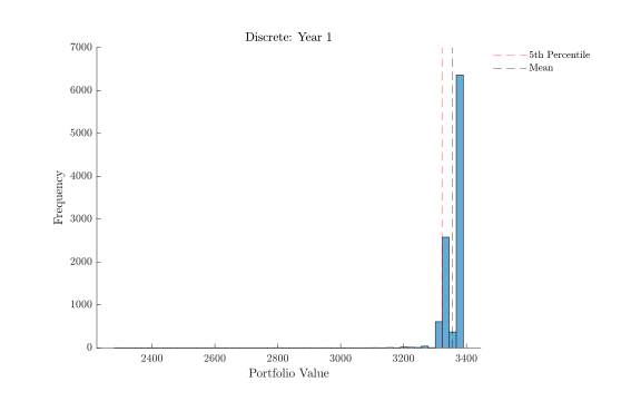
Over a 1-year horizon, the 95% Credit VaR indicates that the portfolio will not lose more than $33.57 with 95% confidence. Extended across 10 years, the continuous model generated Credit VaR estimates that were 7.55% higher on average than the discrete model.